Views: 0 Author: Site Editor Publish Time: 2026-10-14 Origin: Site
Troubleshooting a newly installed fiber optic link can quickly become a demanding task. Everything often appears perfectly fine on the main stretch. Yet, a critical high-loss fault goes completely unnoticed because it hides right at the beginning of the cable. This frustrating scenario is a common and costly reality for network technicians and field engineers. The primary diagnostic tool used to prevent these measurement blind spots is the Optical Time Domain Reflectometer. While this instrument is incredibly powerful and serves as the ultimate tool for network certification, it possesses a fundamental physical limitation known as the dead zone.
To accurately read a trace and ensure long-term network reliability, field engineers must grasp the critical differences between an event dead zone and an attenuation dead zone. This comprehensive guide breaks down these complex optical phenomena into clear, objective, and highly actionable concepts. Mastering these principles empowers you to execute flawless network certifications and avoid costly truck rolls.
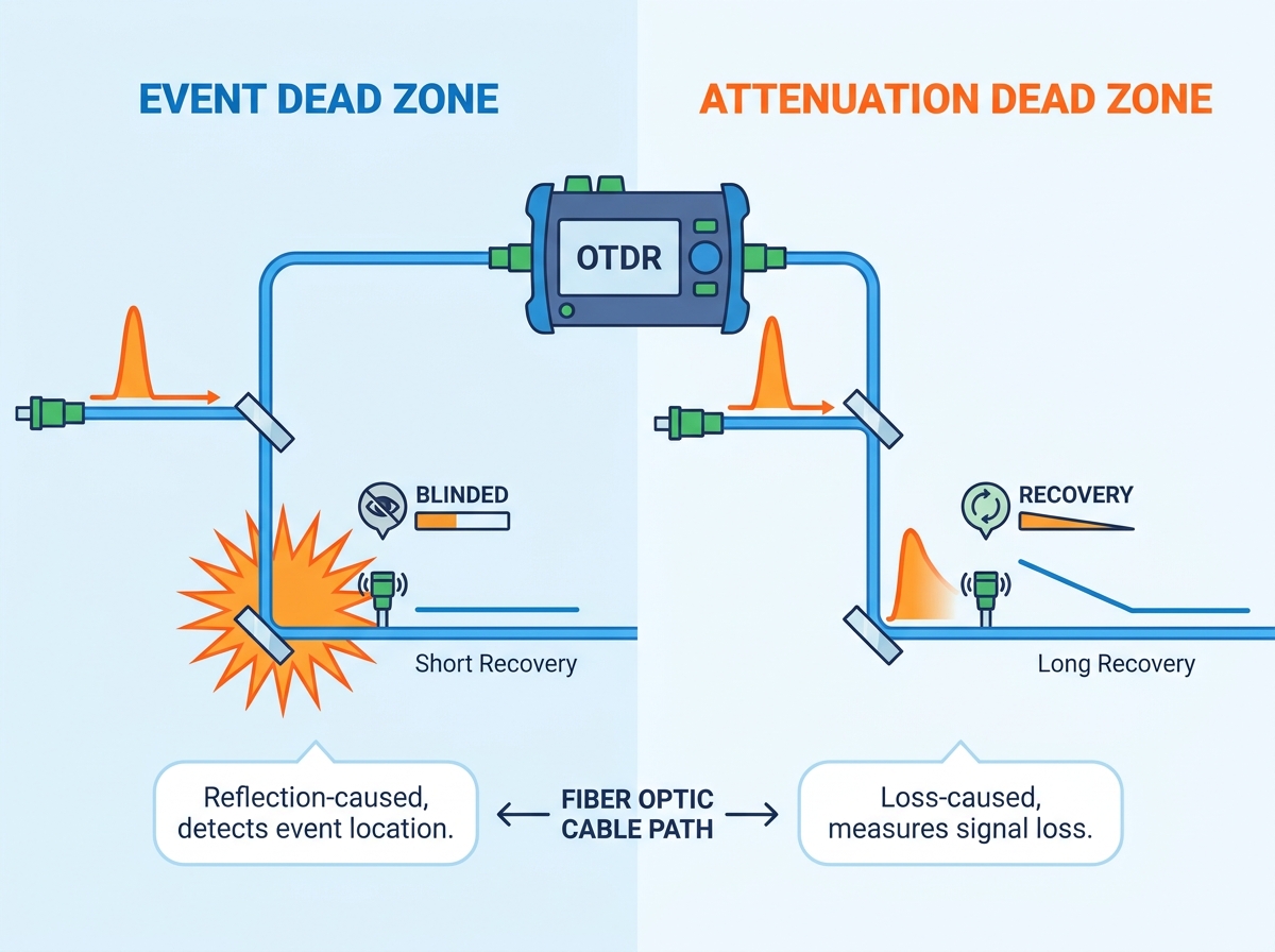
An Optical Time Domain Reflectometer utilizes targeted light pulses to map fiber optic cables and locate faults. However, high-intensity reflections can temporarily blind the internal sensor, resulting in a measurement blind spot.
The Event Dead Zone defines the absolute minimum distance required after a highly reflective event for the equipment to detect another consecutive reflective event, like two closely spaced patch panel connectors.
The Attenuation Dead Zone is the minimum spatial distance required after a reflective event for the device to accurately measure the signal loss of a subsequent non-reflective event, like a fusion splice.
Strategically adjusting the pulse width and integrating a launch cable are the most empirically proven methods to mitigate the negative impact of these limitations during network testing.
To fully comprehend the complexities of measurement blind spots, one must first establish a solid foundational understanding of the primary testing instrument itself. This device is the premier diagnostic tool utilized by telecommunications professionals to characterize optical fibers, measure signal loss, and pinpoint the exact geographical location of structural faults.
The operational mechanics of this device rely on fundamental optical physics. The instrument injects a precisely timed, short burst of laser light into one end of the fiber optic cable under test. As this optical energy travels down the glass core, the vast majority of the photons continue forward. However, a microscopic fraction of the light continuously bounces back toward the source due to a natural phenomenon known as Rayleigh backscattering.
Simultaneously, when the light pulse encounters a sudden change in the index of refraction, a much stronger reflection occurs directly back toward the source. This refractive change could be an air gap at a mechanical connector, a dirty end-face, or a physical fracture. This intense return signal is known as a Fresnel reflection. The instrument’s internal photodetector continuously captures this returning light. By calculating the exact time it takes for the backscattered and reflected light to return, the equipment plots a highly accurate visual map. This trace graphs the physical distance on the horizontal axis against the signal power loss on the vertical axis.
In modern optical networks, simple continuity testing with a visual fault locator is entirely insufficient. Executing advanced trace analysis is critical for bottom-of-funnel decision-making and Tier 2 fiber certification. It provides the empirical data required to verify the quality of new fiber installations. Furthermore, it ensures that splice insertion losses fall within strict optical budgets and rapidly locates catastrophic breaks or micro-bends that threaten data transmission reliability.
Even the most advanced testing instruments are bound by the unchangeable laws of optical physics. A dead zone is a specific length of fiber where the instrument is temporarily unable to accurately detect anomalies or measure optical loss.
To conceptualize this, imagine walking into a completely dark room and having someone take a photograph of you with a powerful, blinding flash. For several seconds after the flash fires, your retinas are overwhelmed by the intense burst of light. You are left temporarily blind to the details of the room. A dead zone operates on a nearly identical principle inside the testing equipment.
Fresnel reflections are the primary catalyst for these measurement blind spots. Whenever light passes between two materials with differing refractive indices, a strong reflection occurs. A classic example is light moving from the glass core into the microscopic air gap of a mated connector pair. Because the internal sensor is delicately calibrated to measure the incredibly faint, continuous stream of Rayleigh backscatter, this sudden, high-energy spike completely saturates the highly sensitive photodetector.
The precise time required for the sensor voltage to drop back down to a stable, linear baseline dictates the physical length of the blind spot. Until that internal recovery is complete, the instrument cannot accurately see the normal backscattered light. This effectively hides any potential faults that exist within that specific distance.
The first specific type of blind spot that field technicians must account for is the Event Dead Zone. This metric is absolutely critical for high-density fiber environments. Hyperscale data centers and Fiber-to-the-Home distribution hubs frequently feature multiple cross-connections spaced closely together.
From a highly technical standpoint, the event dead zone is defined as the minimum physical distance required from the beginning of a reflective event to the point where the receiver recovers sufficiently to detect the presence of another consecutive reflective event. According to standard industry protocols like Telcordia, this recovery threshold is typically measured at 1.5 dB below the absolute peak amplitude of the initial reflection. Within this specific zone, the instrument can acknowledge that a second physical event exists. However, it cannot accurately measure its loss. It simply registers a second spike on the trace.
Consider a real-world field scenario. You are certifying a fiber link where two equipment racks are connected by patch panels situated exactly two meters apart. If your instrument parameters yield an event dead zone of three meters, the receiver will not have recovered from the first panel reflection before the light hits the second. Consequently, the generated trace will merge both physical reflections, displaying them as a single, elongated anomaly. Precise fault isolation becomes virtually impossible under these conditions.
When analyzing a standard trace graph, an event dead zone is visually distinct at the site of any Fresnel reflection. You will immediately observe a sharp, nearly vertical spike indicating the reflection. Following the peak of this spike, the signal line will drop steeply. The event dead zone concludes at the exact moment on this downward slope where the signal has stabilized just enough to spike upward again, should a second reflective event occur on the line.
While the event dead zone strictly dictates the ability to detect consecutive events, the Attenuation Dead Zone is a far more stringent and demanding metric. It defines the absolute minimum distance required after a reflective event for the instrument to fully recover and accurately measure the signal attenuation of a subsequent non-reflective event.
Industry standards dictate that the attenuation dead zone officially ends when the receiver has recovered to within 0.5 dB of the normal, linear backscatter baseline. Measuring a microscopic drop in optical power requires the photodetector to be perfectly stable. Therefore, the attenuation dead zone is universally longer than the event dead zone across all testing platforms. The internal sensor simply needs significantly more physical distance along the fiber to settle back to its precise baseline compared to merely detecting another massive reflective spike.
Understanding this specific zone is paramount for quality control during complex splicing operations. Imagine a technician installs a mechanical connector and then performs a high-quality fusion splice just three meters down the line to attach a pigtail. If the instrument features an attenuation dead zone of five meters, the fusion splice falls entirely within the recovery tail of the connector reflection.
In this scenario, the device will be completely unable to calculate the precise insertion loss of that fusion splice. The trace will clearly show the reflection of the connector, and the slope will eventually stabilize. However, the tiny step down representing the splice loss will be swallowed by the dead zone. Without an accurate decibel reading, the technician cannot definitively pass or fail the splice quality. This oversight potentially leaves a high-loss fault hidden in the active network.
Looking at current industry trajectories, the rapid deployment of 5G networks and high-density optical architectures is pushing loss budgets to their absolute limits. The physical distance between passive optical components is shrinking to mere centimeters. Consequently, telecommunications analysts note a surging demand for fiber optic testing equipment capable of ultra-short dead zones. Field engineers now require advanced platforms capable of resolving discrete events separated by minimal fiber lengths. Furthermore, the integration of algorithmic and AI-driven trace analysis is rapidly becoming a standard expectation, assisting operators in automatically distinguishing between these two zones without tedious manual cursor placement.
For network engineers and procurement teams evaluating testing equipment, misinterpreting these two specifications can lead to purchasing an inadequate instrument. When evaluating gear, professionals look for specifications similar to Skycom models, which frequently feature an event dead zone as tight as 0.5 meters and an attenuation dead zone of 2.5 meters. These parameters are non-negotiable for modern high-density panel certification.
The fundamental distinction between the two zones lies in the measurement objective. The event dead zone is strictly about spatial resolution and detection. Can the device physically see two distinct connectors? In contrast, the attenuation dead zone is about quantification. Can the device accurately measure the optical loss of a component placed immediately after a reflection? Because of the rigorous stabilization requirements of the photodiode, the length of the attenuation dead zone will always exceed that of the event dead zone under identical testing parameters.
Feature | Event Dead Zone | Attenuation Dead Zone |
|---|---|---|
Technical Definition | Minimum distance required to detect the next consecutive reflective event. | Minimum distance required to accurately measure the loss of the next event. |
Measurement Threshold | Typically measured at 1.5 dB below the initial reflection peak. | Typically measured at 0.5 dB from the linear backscatter baseline. |
Typical Distance | Shorter, ranging from 0.5m to 2m on modern, high-quality devices. | Longer, ranging from 2.5m to 5m depending on the selected pulse width. |
Primary Use Case | Locating closely spaced patch panels, mechanical connectors, or physical breaks. | Quantifying the specific insertion loss of fusion splices or macro-bends. |
Trace Appearance | Measured from the peak to the exact start of the next visible upward spike. | Measured from the peak until the trace returns completely to a flat, linear slope. |
While measurement blind spots are ultimately governed by optical physics, the technician operating the equipment has direct control over their severity through the manipulation of testing parameters. The most impactful setting on the device is the pulse width. This metric dictates the duration of the laser burst injected into the fiber, typically measured in nanoseconds or microseconds. The physical length of the light pulse traveling through the fiber is directly proportional to the duration of the burst.
Selecting the correct pulse width requires a delicate balance between spatial resolution and dynamic range. Dynamic range refers to the maximum optical distance the instrument can accurately analyze. Understanding this balance is critical for field engineers tackling diverse testing scenarios.
Configuring the equipment to emit a shorter pulse of light, like 3 to 10 nanoseconds, directly results in a brief reflection. This allows the photodetector to recover rapidly. It produces the shortest possible dead zones, thereby providing exceptionally high spatial resolution. Short pulses are strictly ideal for resolving closely spaced events in short links, such as enterprise LANs or drop cables. However, shorter pulses inject significantly less optical energy into the core. They cannot travel long distances before being absorbed, resulting in a severely limited dynamic range.
In contrast, utilizing a long pulse width, like 1000 to 20,000 nanoseconds, injects a massive amount of optical energy into the fiber. This high energy allows the signal to travel across long-haul telecommunications networks, providing a robust dynamic range. The inevitable trade-off is that a longer pulse creates a physically longer reflection. The photodetector remains saturated for an extended period. This creates massive dead zones that can stretch for tens or even hundreds of meters, completely obscuring any near-end events.
Since these optical blind spots are an unavoidable reality, fiber optic professionals utilize specific hardware accessories and optimized testing protocols to effectively mitigate their impact during certification.
The most empirically effective hardware solution is the deployment of a launch cable, frequently referred to in the industry as a dead zone eliminator or a dummy fiber. This accessory is a spool of high-quality fiber optic cable housed in a protective box. It connects directly between the testing equipment and the actual network fiber under test.
When the initial laser pulse is fired, the very first mechanical connection inherently generates a massive reflection. Because the instrument is located at distance zero, the resulting dead zone obscures the first few meters of the network. Measuring the insertion loss of that initial connector becomes impossible. By utilizing a launch cable, this unavoidable blind spot is captured entirely within the spool of the dummy fiber. By the time the light pulse reaches the first connector of the actual network, the photodetector has fully stabilized. The operator can now accurately measure its loss. For comprehensive bidirectional testing, a receive cable is similarly placed at the far end of the link.
Beyond hardware additions, optimizing the physical connections is an absolute necessity. Technicians must ensure that all fiber end-faces are impeccably clean before mating. Microscopic dirt, dust, or skin oils on a connector drastically increase optical reflectance. Higher reflectance equals a longer saturation time for the detector, which proportionally elongates the dead zone. Strict dry and wet cleaning protocols, utilizing lint-free wipes and specialized optical solvents, must be rigorously followed.
Specifically, utilizing Angled Physical Contact connectors instead of standard Ultra Physical Contact connectors wherever network architecture permits can drastically reduce Fresnel reflections. The 8-degree angled end-face of an angled ferrule forces backscattered light out into the fiber cladding rather than allowing it to return straight down the core to the detector. This minimizes sensor saturation and physically shrinks the resulting dead zone.
Translating the theoretical physics of dead zones into practical trace analysis requires a systematic, objective approach. A trace is a linear representation of the fiber structural health. Accurately deciphering its slopes and anomalies is the hallmark of a skilled field technician.
When reviewing a trace on the display, professionals methodically scan the data sequentially from left to right. They categorize events based on their visual signatures while actively factoring in pulse width parameters.
Components like mechanical connectors, patch panels, or physical fractures manifest as sharp, vertical spikes on the trace. When reading these reflective events, the technician must carefully examine the downward slope immediately following the spike. This determines if an attenuation dead zone is hiding a subsequent fault.
High-quality fusion splices or macro-bends appear as sudden, small vertical steps down in the linear trace. They show no accompanying upward spike. Because they do not cause significant reflection, they do not create dead zones themselves. However, their accurate measurement is entirely dependent on whether they fall within the attenuation dead zone of a preceding reflective event.
Finally, the physical end of the link is characteristically marked by a final, massive reflective spike. This is followed by an immediate, vertical drop into a jagged pattern known as the noise floor. The signal has exhausted its energy, and the instrument is simply reading background static.
Dead zones remain an unavoidable physical reality in fiber optic testing, governed by the absolute laws of light reflection and sensor saturation. However, knowing the fundamental difference between event and attenuation zones ensures highly accurate network analysis and prevents costly misdiagnoses. By mastering pulse width adjustments and consistently deploying launch cables, technicians can effectively bypass these limitations in the field.
Ultimately, investing in high-quality OTDRs equipped with ultra-short dead zone specifications, paired with a rigorous understanding of trace analysis, is the true hallmark of a professional fiber optic technician. Equip yourself with the right knowledge and robust equipment from trusted brands like Skycom, and no hidden fault will ever go unnoticed in your network deployments.
Dynamic range refers to the maximum optical distance the equipment can accurately analyze down a fiber link; it measures the overall signal reach. The dead zone, conversely, is the temporary measurement blind spot created by strong optical reflections near the testing source. These two critical metrics share an inverse relationship heavily dependent on pulse width. Increasing the pulse width improves the dynamic range so the light travels further, but it simultaneously increases the physical length of the dead zone.
The required length of a dummy fiber depends entirely on the specific pulse width configured for your test. As a general industry standard for field applications, a 150-meter to 1-kilometer launch cable is utilized. The fundamental empirical rule is that the launch cable must be physically longer than the specific attenuation dead zone of the testing equipment at the selected pulse width. This ensures the sensor recovers before the actual network begins.
No, it cannot be entirely eliminated because it is a direct result of the fundamental laws of optical physics and the natural saturation limits of photodiodes. However, its negative impact can be heavily minimized by utilizing the shortest possible pulse widths and ensuring impeccable end-face cleanliness on angled connectors. Furthermore, the initial blind spot can be effectively bypassed for the network under test by deploying a dead zone eliminator.
Modern, high-tier testing devices feature incredibly sensitive and fast-recovering photodetectors, achieving event dead zones as remarkably small as 0.5 to 1 meter. This level of optical precision is considered excellent. It is highly recommended for certifying short-run infrastructure, including FTTx deployments, local area networks, or dense data center environments where cross-connects are spaced very closely together.
Testing the dead zone of your equipment involves connecting a short patch cord of known length between the instrument port and a highly reflective event, like an open PC connector. By setting the device to its shortest pulse width and firing a trace, you can measure the distance from the peak of the initial reflection to the point where the signal drops 1.5 dB for the event dead zone, or returns to the linear baseline for the attenuation dead zone.
High reflectance is primarily caused by a severe change in the refractive index within the optical path. In field environments, the most common culprits are dirty connector end-faces, poorly mated mechanical connections leaving a microscopic air gap, shattered glass cores from physical cable damage, or utilizing mismatched connector polish types, such as mating an APC to a UPC connector.